12  Comparison of TransPropy with Other Tool Packages Using GSEA (Gene: CFD)

library(readr)
library(TransProR)
library(dplyr)
library(rlang)
library(linkET)
library(funkyheatmap)
library(tidyverse)
library(RColorBrewer)
library(ggalluvial)
library(tidyr)
library(tibble)
library(ggplot2)
library(ggridges)
library(GSVA)
library(fgsea) 
library(clusterProfiler)
library(enrichplot)
library(MetaTrx)

12.1 CFD

12.1.1 correlation_TransPropy_CFD

12.1.1.1 HALLMARKS

# Create a named vector from the correlation data
geneList <- correlation_TransPropy_CFD$cor
names(geneList) = correlation_TransPropy_CFD$gene2
geneList = sort(geneList, decreasing = TRUE)
head(geneList)

# Read the hallmark gene sets
hallmarks <- read.gmt("h.all.v7.4.symbols.gmt")

# Perform Gene Set Enrichment Analysis (GSEA)
TransPropy_CFD_hallmarks_y <- GSEA(geneList, TERM2GENE = hallmarks, pvalueCutoff = 0.05)

# Sort the results by NES (Normalized Enrichment Score)
TransPropysorted_df <- TransPropy_CFD_hallmarks_y@result %>% arrange(desc(NES))

# Count the number of core enriched genes in each row
TransPropysorted_df$core_gene_count <- sapply(strsplit(as.character(TransPropysorted_df$core_enrichment), "/"), length)

# Define a function to process strings (change pathway name prefixes and case)
process_string <- function(s) {
  # Remove the first word and underscore
  s <- sub("^HALLMARK_", "", s)
  # Split the string by underscore
  words <- unlist(strsplit(s, "_"))
  # Capitalize the first letter of each word and make other letters lowercase
  words <- tolower(words)
  words <- paste(toupper(substring(words, 1, 1)), substring(words, 2), sep = "")
  # Combine the words back into a single string
  result <- paste(words, collapse = " ")
  return(result)
}

# Apply the function to the ID and Description columns
TransPropysorted_df$ID <- sapply(TransPropysorted_df$ID, process_string)
TransPropysorted_df$Description <- sapply(TransPropysorted_df$Description, process_string)

# Process the row names
rownames(TransPropysorted_df) <- sapply(rownames(TransPropysorted_df), process_string)

# Display the results
print(TransPropysorted_df)

# Assign the processed data back to y@result for the GSEA collective pathway plot
TransPropy_CFD_hallmarks_y@result <- TransPropysorted_df

# Process y@geneSets for the GSEA collective pathway plot
# Get the current geneSet names
gene_set_names <- names(TransPropy_CFD_hallmarks_y@geneSets)
# Apply the process_string function to the names
new_gene_set_names <- sapply(gene_set_names, process_string)
# Update the geneSet names
names(TransPropy_CFD_hallmarks_y@geneSets) <- new_gene_set_names
# Display the modified geneSet names
print(names(TransPropy_CFD_hallmarks_y@geneSets))


print(TransPropy_CFD_hallmarks_y@result$ID)
# Set the color palette for the plot
color = colorRampPalette(c("#6a1b9a", "#00838f"))(9)

# Plot all gene sets in one image
new_gseaNb(object = TransPropy_CFD_hallmarks_y,
            geneSetID = c("Xenobiotic Metabolism",
                          "Kras Signaling Dn",
                          "Myogenesis",
                          "Allograft Rejection",  
                          "Glycolysis",
                          "Spermatogenesis",
                          "Mitotic Spindle",
                          "E2f Targets",          
                          "G2m Checkpoint"
            ),
            curveCol = color,
            lineSize = 2.5,            # Control the line size in the first plot
            lineAlpha = 0.6,           # Control the line transparency in the first plot
            segmentSize = 3,           # Control the vertical line size in the second plot
            segmentAlpha = 0.6,        # Control the vertical line transparency in the second plot
            plotHeightRatio = c(0.3, 0.5, 0.2),  # Control the height ratio of the three plots
            legend.position = "none",
            htCol = rev(c("#6a1b9a", "#00838f")), 
            rankCol = rev(c("#6a1b9a", "white", "#00838f"))
)

TransPropy_CFD_hallmarks_GSEA_legend

12.1.1.2 KEGG

# KEGG
kegg <- read.gmt("c2.cp.kegg.v7.4.symbols.gmt")

TransPropy_CFD_kegg_y <- GSEA(geneList, TERM2GENE = kegg)

# Sort by NES (Normalized Enrichment Score)
TransPropysorted_df <- TransPropy_CFD_kegg_y@result %>% arrange(desc(NES))

# Count the number of core enriched genes in each row
TransPropysorted_df$core_gene_count <- sapply(strsplit(as.character(TransPropysorted_df$core_enrichment), "/"), length)

# Define a function to process strings (change pathway name prefixes and case)
process_string <- function(s) {
  # Remove the first word and underscore
  s <- sub("^KEGG_", "", s)
  # Split the string by underscore
  words <- unlist(strsplit(s, "_"))
  # Capitalize the first letter of each word and make other letters lowercase
  words <- tolower(words)
  words <- paste(toupper(substring(words, 1, 1)), substring(words, 2), sep = "")
  # Combine the words back into a single string
  result <- paste(words, collapse = " ")
  return(result)
}

# Apply the function to the ID and Description columns
TransPropysorted_df$ID <- sapply(TransPropysorted_df$ID, process_string)
TransPropysorted_df$Description <- sapply(TransPropysorted_df$Description, process_string)

# Process the row names
rownames(TransPropysorted_df) <- sapply(rownames(TransPropysorted_df), process_string)

# Display the results
print(TransPropysorted_df)

# Assign the processed data back to y@result for the GSEA collective pathway plot
TransPropy_CFD_kegg_y@result <- TransPropysorted_df

# Process y@geneSets for the GSEA collective pathway plot
# Get the current geneSet names
gene_set_names <- names(TransPropy_CFD_kegg_y@geneSets)
# Apply the process_string function to the names
new_gene_set_names <- sapply(gene_set_names, process_string)
# Update the geneSet names
names(TransPropy_CFD_kegg_y@geneSets) <- new_gene_set_names

# Display the modified geneSet names
print(names(TransPropy_CFD_kegg_y@geneSets))

# Save the processed results to a CSV file
# write.table(TransPropy_CFD_kegg_y@result, file="Transpropy_KEGG_GSEA_all.csv", sep=",", row.names=TRUE)

print(TransPropy_CFD_kegg_y@result$ID)
# Set the color palette for the plot
color = colorRampPalette(c("#6a1b9a", "#00838f"))(14)

# Plot all gene sets in one image
new_gseaNb(object = TransPropy_CFD_kegg_y,
            geneSetID = c("Metabolism Of Xenobiotics By Cytochrome P450",
                          "Drug Metabolism Cytochrome P450",             
                          "Retinol Metabolism",
                          "Arachidonic Acid Metabolism",                 
                          "Calcium Signaling Pathway",
                          "Ppar Signaling Pathway",                      
                          "Vascular Smooth Muscle Contraction",
                          "Glycolysis Gluconeogenesis",                  
                          "Endocytosis",
                          "Type I Diabetes Mellitus",                    
                          "Hematopoietic Cell Lineage",
                          "Graft Versus Host Disease",                   
                          "Leishmania Infection",
                          "Cell Cycle"), 
            curveCol = color,
            lineSize = 2.5,            # Control the line size in the first plot
            lineAlpha = 0.6,           # Control the line transparency in the first plot
            segmentSize = 3,           # Control the vertical line size in the second plot
            segmentAlpha = 0.6,        # Control the vertical line transparency in the second plot
            plotHeightRatio = c(0.3, 0.5, 0.2),  # Control the height ratio of the three plots
            # legend.position = "none",
            htCol = rev(c("#6a1b9a", "#00838f")), 
            rankCol = rev(c("#6a1b9a", "white", "#00838f"))
)

TransPropy_CFD_kegg_GSEA_legend

12.1.2 correlation_deseq2_CFD

12.1.2.1 HALLMARKS

# Create a named vector from the correlation data
geneList <- correlation_deseq2_CFD$cor
names(geneList) = correlation_deseq2_CFD$gene2
geneList = sort(geneList, decreasing = TRUE)
head(geneList)

# Read the hallmark gene sets
hallmarks <- read.gmt("h.all.v7.4.symbols.gmt")

# Perform Gene Set Enrichment Analysis (GSEA)
deseq2_CFD_hallmarks_y <- GSEA(geneList, TERM2GENE = hallmarks, pvalueCutoff = 0.05)

# Sort the results by NES (Normalized Enrichment Score)
deseq2sorted_df <- deseq2_CFD_hallmarks_y@result %>% arrange(desc(NES))

# Count the number of core enriched genes in each row
deseq2sorted_df$core_gene_count <- sapply(strsplit(as.character(deseq2sorted_df$core_enrichment), "/"), length)

# Define a function to process strings (change pathway name prefixes and case)
process_string <- function(s) {
  # Remove the first word and underscore
  s <- sub("^HALLMARK_", "", s)
  # Split the string by underscore
  words <- unlist(strsplit(s, "_"))
  # Capitalize the first letter of each word and make other letters lowercase
  words <- tolower(words)
  words <- paste(toupper(substring(words, 1, 1)), substring(words, 2), sep = "")
  # Combine the words back into a single string
  result <- paste(words, collapse = " ")
  return(result)
}

# Apply the function to the ID and Description columns
deseq2sorted_df$ID <- sapply(deseq2sorted_df$ID, process_string)
deseq2sorted_df$Description <- sapply(deseq2sorted_df$Description, process_string)

# Process the row names
rownames(deseq2sorted_df) <- sapply(rownames(deseq2sorted_df), process_string)

# Display the results
print(deseq2sorted_df)

# Assign the processed data back to y@result for the GSEA collective pathway plot
deseq2_CFD_hallmarks_y@result <- deseq2sorted_df

# Process y@geneSets for the GSEA collective pathway plot
# Get the current geneSet names
gene_set_names <- names(deseq2_CFD_hallmarks_y@geneSets)
# Apply the process_string function to the names
new_gene_set_names <- sapply(gene_set_names, process_string)
# Update the geneSet names
names(deseq2_CFD_hallmarks_y@geneSets) <- new_gene_set_names

# Display the modified geneSet names
print(names(deseq2_CFD_hallmarks_y@geneSets))

# Save the processed results to a CSV file
# write.table(deseq2sorted_df, file="TransPropy_HALLMARKS_GSEA_all.csv", sep=",", row.names=FALSE)

print(deseq2_CFD_hallmarks_y@result$ID)
# Set the color palette for the plot
color = colorRampPalette(c("#4527a0", "#00695c"))(7)

# Plot all gene sets in one image
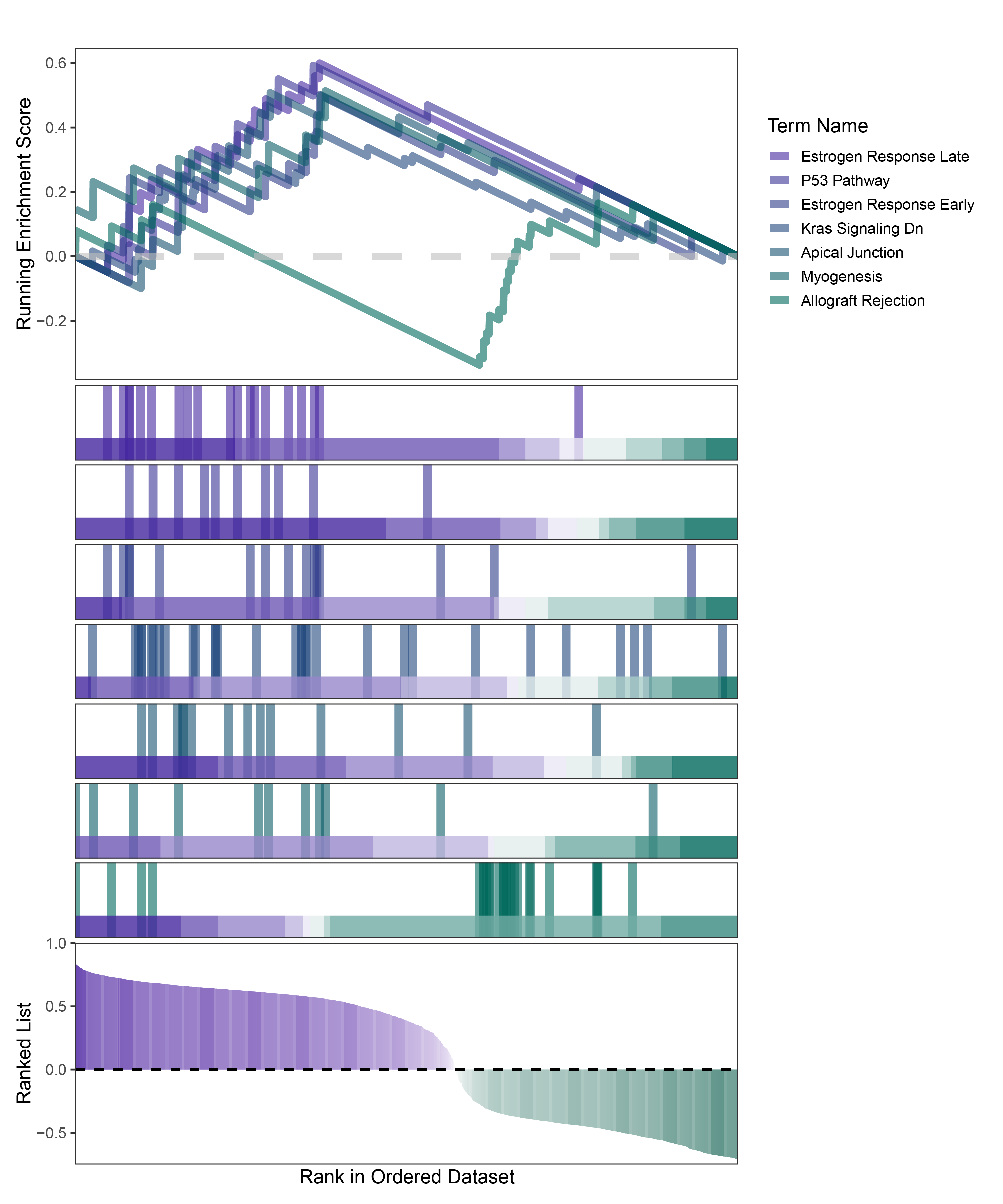
new_gseaNb(object = deseq2_CFD_hallmarks_y,
            geneSetID = c("Estrogen Response Late",
                          "P53 Pathway",
                          "Estrogen Response Early",
                          "Kras Signaling Dn", 
                          "Apical Junction", 
                          "Myogenesis",             
                          "Allograft Rejection"),
            curveCol = color,
            lineSize = 2.5,            # Control the line size in the first plot
            lineAlpha = 0.6,           # Control the line transparency in the first plot
            segmentSize = 3,           # Control the vertical line size in the second plot
            segmentAlpha = 0.6,        # Control the vertical line transparency in the second plot
            plotHeightRatio = c(0.3, 0.5, 0.2),  # Control the height ratio of the three plots
            # legend.position = "none",
            htCol = rev(c("#4527a0", "#00695c")), 
            rankCol = rev(c("#4527a0", "white", "#00695c"))
)

deseq2_CFD_hallmarks_GSEA_legend

12.1.2.2 kegg

#kegg
kegg <- read.gmt("c2.cp.kegg.v7.4.symbols.gmt")

deseq2_CFD_kegg_y <- GSEA(geneList,TERM2GENE =kegg)

# Sort by NES
deseq2sorted_df <- deseq2_CFD_kegg_y@result %>% arrange(desc(NES))
# Count the number of core enrichment genes per row
deseq2sorted_df$core_gene_count <- sapply(strsplit(as.character(deseq2sorted_df$core_enrichment), "/"), length)

# Define a function to process strings (change pathway name prefix and case)
process_string <- function(s) {
  # Remove the first word and underscore at the beginning
  s <- sub("^KEGG_", "", s)
  # Split the string by underscores
  words <- unlist(strsplit(s, "_"))
  # Capitalize the first letter of each word and make the rest lowercase
  words <- tolower(words)
  words <- paste(toupper(substring(words, 1, 1)), substring(words, 2), sep = "")
  # Combine the words
  result <- paste(words, collapse = " ")
  return(result)
}

# Apply the function to the ID and Description columns
deseq2sorted_df$ID <- sapply(deseq2sorted_df$ID, process_string)
deseq2sorted_df$Description <- sapply(deseq2sorted_df$Description, process_string)
# Process row names
rownames(deseq2sorted_df) <- sapply(rownames(deseq2sorted_df), process_string)
# Display the result
print(deseq2sorted_df)

# Transfer the processed data back to y@result for the GSEA collective pathway plot
deseq2_CFD_kegg_y@result <- deseq2sorted_df

# Process y@geneSets for the GSEA collective pathway plot
# Get the current geneSets names
gene_set_names <- names(deseq2_CFD_kegg_y@geneSets)
# Apply the process_string function to the names
new_gene_set_names <- sapply(gene_set_names, process_string)
# Update the geneSets names
names(deseq2_CFD_kegg_y@geneSets) <- new_gene_set_names
# Display the modified geneSets names
print(names(deseq2_CFD_kegg_y@geneSets))

# write.table(y@result, file="Transpropy_KEGG_GSEA_all.csv",sep=",",row.names=T)


print(deseq2_CFD_kegg_y@result$ID)
color = colorRampPalette(c("#4527a0","#00695c"))(7)

# All plot one image
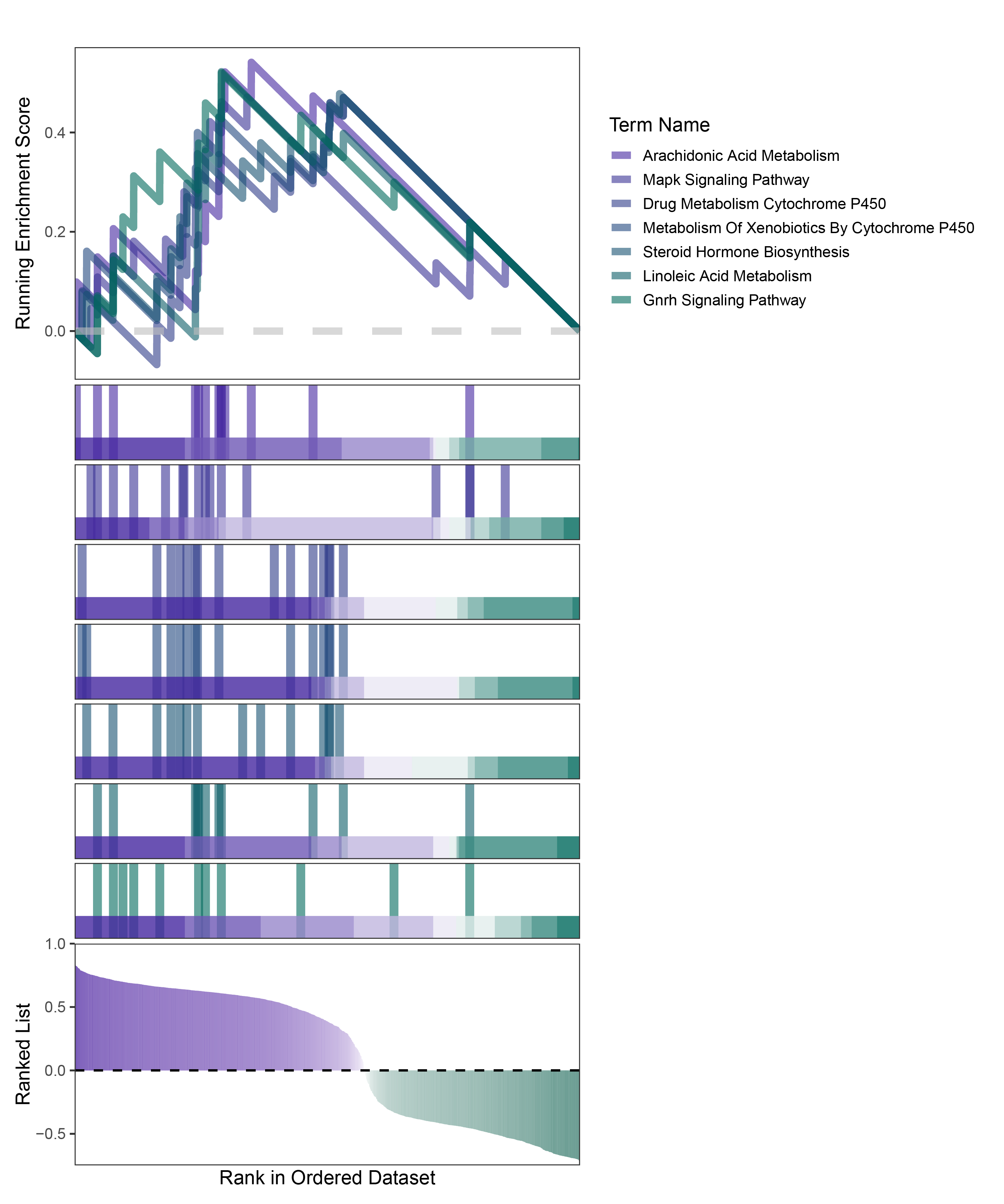
new_gseaNb(object = deseq2_CFD_kegg_y,
            geneSetID = c("Arachidonic Acid Metabolism",
                          "Mapk Signaling Pathway",                      
                          "Drug Metabolism Cytochrome P450",
                          "Metabolism Of Xenobiotics By Cytochrome P450",
                          "Steroid Hormone Biosynthesis",
                          "Linoleic Acid Metabolism",                    
                          "Gnrh Signaling Pathway"
                          ), 
            curveCol = color,
            lineSize = 2.5,            # Control the size of the lines in the first plot
            lineAlpha = 0.6,         # Control the transparency of the lines in the first plot
            segmentSize = 3,       # Control the size of the vertical lines in the second plot
            segmentAlpha = 0.6,      # Control the transparency of the vertical lines in the second plot
            plotHeightRatio = c(0.3, 0.5, 0.2),  # Control the vertical proportions of the three plots
            #legend.position = "none",
            htCol = rev(c("#4527a0","#00695c")), 
            rankCol = rev(c("#4527a0","white","#00695c"))
)

deseq2_CFD_kegg_GSEA_legend

12.1.3 correlation_edgeR_CFD

12.1.3.1 HALLMARKS

# Translate the gene list from the correlation_edgeR_CFD data
geneList <- correlation_edgeR_CFD$cor
names(geneList) = correlation_edgeR_CFD$gene2
geneList = sort(geneList, decreasing = TRUE)
head(geneList)

# Read hallmark gene sets
hallmarks <- read.gmt("h.all.v7.4.symbols.gmt")
edgeR_CFD_hallmarks_y <- GSEA(geneList, TERM2GENE = hallmarks, pvalueCutoff = 0.05)
# Sort by Normalized Enrichment Score (NES)
edgeRsorted_df <- edgeR_CFD_hallmarks_y@result %>% arrange(desc(NES))
# Count core enrichment genes per pathway
edgeRsorted_df$core_gene_count <- sapply(strsplit(as.character(edgeRsorted_df$core_enrichment), "/"), length)

# Define a function to modify string (change pathway name prefix and casing)
process_string <- function(s) {
  # Remove the first word and underscore
  s <- sub("^HALLMARK_", "", s)
  # Split the string on underscores
  words <- unlist(strsplit(s, "_"))
  # Capitalize the first letter of each word, rest lowercase
  words <- tolower(words)
  words <- paste(toupper(substring(words, 1, 1)), substring(words, 2), sep = "")
  # Concatenate the words
  result <- paste(words, collapse = " ")
  return(result)
}

# Apply the function to ID and Description columns
edgeRsorted_df$ID <- sapply(edgeRsorted_df$ID, process_string)
edgeRsorted_df$Description <- sapply(edgeRsorted_df$Description, process_string)
# Modify row names
rownames(edgeRsorted_df) <- sapply(rownames(edgeRsorted_df), process_string)
# Display the modified dataframe
print(edgeRsorted_df)

# Update processed data back to y@result for a collective GSEA pathway diagram
edgeR_CFD_hallmarks_y@result <- edgeRsorted_df

# Process y@geneSets for collective pathway diagrams
# Get current geneSets names
gene_set_names <- names(edgeR_CFD_hallmarks_y@geneSets)
# Apply process_string function to names
new_gene_set_names <- sapply(gene_set_names, process_string)
# Update geneSets names
names(edgeR_CFD_hallmarks_y@geneSets) <- new_gene_based_names
# Display updated geneSets names
print(names(edgeR_CFD_hallmarks_y@geneSets))

print(edgeR_CFD_hallmarks_y@result$ID)
# Generate GSEA plots for selected gene sets
color = colorRampPalette(c("#283593","#2e7d32"))(5)

# Plot all on one image
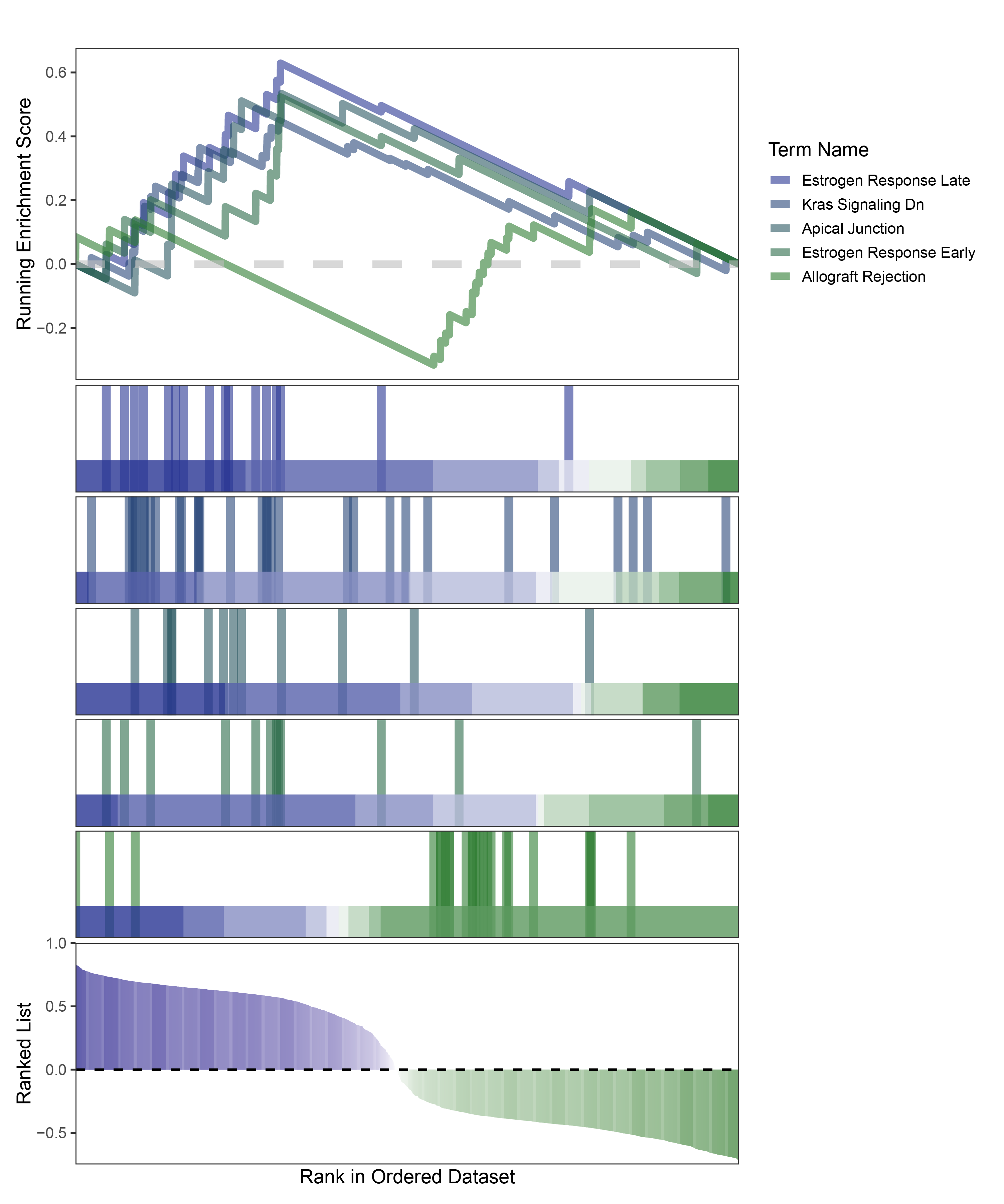
new_gseaNb(object = edgeR_CFD_hallmarks_y,
            geneSetID = c("Estrogen Response Late",
                          "Kras Signaling Dn",
                          "Apical Junction",
                          "Estrogen Response Early",
                          "Allograft Rejection"),
            curveCol = color,
            lineSize = 2.5,            # Control the size of the first plot's lines
            lineAlpha = 0.6,         # Control the transparency of the first plot's lines
            segmentSize = 3,       # Control the size of the second plot's vertical lines
            segmentAlpha = 0.6,      # Control the transparency of the second plot's vertical lines
            plotHeightRatio = c(0.3, 0.5, 0.2),  # Control the proportion of the three plots
            #legend.position = "none",
            htCol = rev(c("#283593","#2e7d32")),
            rankCol = rev(c("#283593","white","#2e7d32"))
)

edgeR_CFD_hallmarks_GESA_legend

12.1.3.2 KEGG

#kegg
kegg <- read.gmt("c2.cp.kegg.v7.4.symbols.gmt")

edgeR_CFD_kegg_y <- GSEA(geneList, TERM2GENE = kegg)

# Sort by NES
edgeRsorted_df <- edgeR_CFD_kegg_y@result %>% arrange(desc(NES))
# Count the number of core enriched genes per row
edgeRsorted_df$core_gene_count <- sapply(strsplit(as.character(edgeRsorted_df$core_enrichment), "/"), length)

# Define a function to process strings (change pathway name prefix and case)
process_string <- function(s) {
  # Remove the first word and underscore at the beginning
  s <- sub("^KEGG_", "", s)
  # Split the string by underscore
  words <- unlist(strsplit(s, "_"))
  # Capitalize the first letter of each word, make other letters lowercase
  words <- tolower(words)
  words <- paste(toupper(substring(words, 1, 1)), substring(words, 2), sep = "")
  # Combine words
  result <- paste(words, collapse = " ")
  return(result)
}

# Apply the function to ID and Description columns
edgeRsorted_df$ID <- sapply(edgeRsorted_df$ID, process_string)
edgeRsorted_df$Description <- sapply(edgeRsorted_df$Description, process_string)
# Process row names
rownames(edgeRsorted_df) <- sapply(rownames(edgeRsorted_df), process_string)
# Display results
print(edgeRsorted_df)

# Send the processed data back to y@result for easy GSEA pathway diagram
edgeR_CFD_kegg_y@result <- edgeRsorted_df

# Process y@geneSets for easy GSEA pathway diagram
# Get the current geneSets names
gene_set_names <- names(edgeR_CFD_kegg_y@geneSets)
# Apply the process_string function to names
new_gene_set_names <- sapply(gene_set_names, process_string)
# Update the names of geneSets
names(edgeR_CFD_kegg_y@geneSets) <- new_gene_set_names
# Display the updated geneSets names
print(names(edgeR_CFD_kegg_y@geneSets))

# Write the result to a CSV file
# write.table(y@result, file="Transpropy_KEGG_GSEA_all.csv", sep=",", row.names=T)

# Display IDs
print(edgeR_CFD_kegg_y@result$ID)
# Define a color gradient
color = colorRampPalette(c("#283593","#2e7d32"))(5)

# Plot all in one image
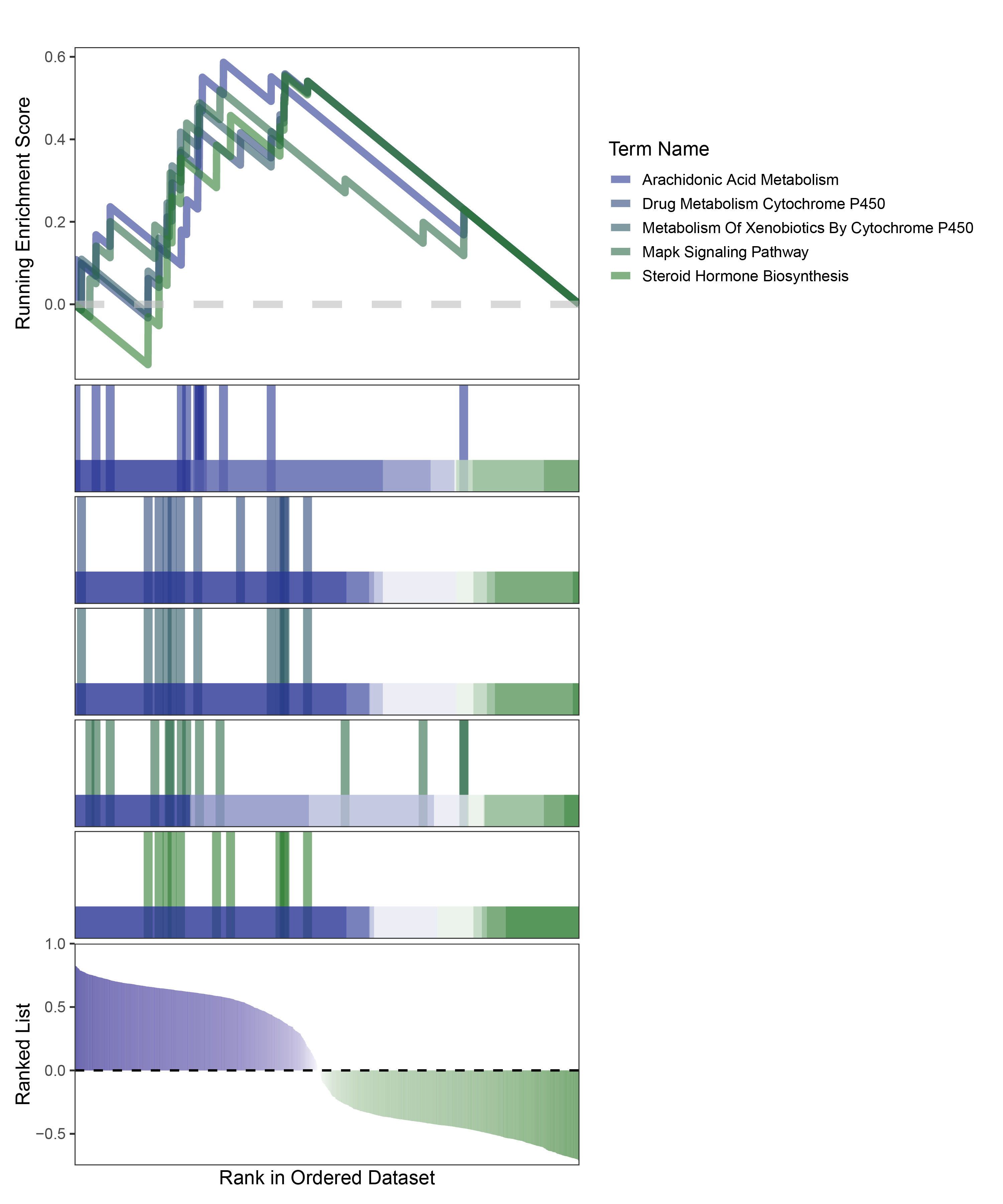
new_gseaNb(object = edgeR_CFD_kegg_y,
            geneSetID = c("Arachidonic Acid Metabolism",
                          "Drug Metabolism Cytochrome P450",
                          "Metabolism Of Xenobiotics By Cytochrome P450",
                          "Mapk Signaling Pathway",
                          "Steroid Hormone Biosynthesis"), 
            curveCol = color,
            lineSize = 2.5,            # Control the line size of the first plot
            lineAlpha = 0.6,         # Control the transparency of the line in the first plot
            segmentSize = 3,       # Control the size of the vertical lines in the second plot
            segment Alpha = 0.6,      # Control the transparency of the vertical lines in the second plot
            plotHeightRatio = c(0.3, 0.5, 0.2),  # Control the height ratio of the three plots
            #legend.position = "none",
            htCol = rev(c("#283593","#2e7d32")), 
            rankCol = rev(c("#283593","white","#2e7d32"))
)

edgeR_CFD_kegg_GESA_legend

12.1.4 correlation_limma_CFD

12.1.4.1 HALLMARKS

geneList <- correlation_limma_CFD$cor
names(geneList) = correlation_limma_CFD$gene2
geneList = sort(geneList, decreasing = TRUE)
head(geneList)

#hallmark
hallmarks <- read.gmt("h.all.v7.4.symbols.gmt")
limma_CFD_hallmarks_y <- GSEA(geneList, TERM2GENE = hallmarks, pvalueCutoff = 0.05)
# Sort by NES
limmasorted_df <- limma_CFD_hallmarks_y@result %>% arrange(desc(NES))
# Count the number of core enriched genes per row
limmasorted_df$core_gene_count <- sapply(strsplit(as.character(limmasorted_df$core_enrichment), "/"), length)

# Define a function to process strings (change pathway name prefix and case)
process_string <- function(s) {
  # Remove the first word and underscore at the beginning
  s <- sub("^HALLMARK_", "", s)
  # Split the string by underscore
  words <- unlist(strsplit(s, "_"))
  # Capitalize the first letter of each word, make other letters lowercase
  words <- tolower(words)
  words <- paste(toupper(substring(words, 1, 1)), substring(words, 2), sep = "")
  # Combine words
  result <- paste(words, collapse = " ")
  return(result)
}

# Apply the function to ID and Description columns
limmasorted_df$ID <- sapply(limmasorted_df$ID, process_string)
limmasorted_df$Description <- sapply(limmasorted_df$Description, process_string)
# Process row names
rownames(limmasorted_df) <- sapply(rownames(limmasorted_df), process_string)
# Display results
print(limmasorted_df)

# Send the processed data back to y@result for easy GSEA pathway diagram
limma_CFD_hallmarks_y@result <- limmasorted_df

# Process y@geneSets for easy GSEA pathway diagram
# Get the current geneSets names
gene_set_names <- names(limma_CFD_hallmarks_y@geneSets)
# Apply the process_string function to names
new_gene_set_names <- sapply(gene_set_names, process_string)
# Update the names of geneSets
names(limma_CFD_hallmarks_y@geneSets) <- new_gene_set<- names
# Display the updated geneSets names
print(names(limma_CFD_hallmarks_y@geneSets))

# Write the result to a CSV file
# write.table(TransPropysorted_df, file="TransPropy_HALLMARKS_GSEA_all.csv", sep=",", row.names=F)


print(limma_CFD_hallmarks_y@result$ID)
# Define a color gradient
color = colorRampPalette(c("#1565c0","#558b2f"))(13)

# Plot all in one image
new_gseaNb(object = limma_CFD_hallmarks_y,
            geneSetID = c("Estrogen Response Late",
                          "Adipogenesis",
                          "P53 Pathway",              
                          "Myogenesis",
                          "Apical Junction",
                          "Mtorc1 Signaling",         
                          "Complement",
                          "Spermatogenesis",
                          "Inflammatory Response",    
                          "Interferon Gamma Response",
                          "Allograft Rejection",
                          "E2f Targets",              
                          "G2m Checkpoint"),
            curveCol = color,
            lineSize = 2.5,            # Control the line size of the first plot
            lineAlpha = 0.6,           # Control the transparency of the line in the first plot
            segmentSize = 3,           # Control the size of the vertical lines in the second plot
            segmentAlpha = 0.6,        # Control the transparency of the vertical lines in the second plot
            plotHeightRatio = c(0.3, 0.5, 0.2),  # Control the height ratio of the three plots
            #legend.position = "none",
            htCol = rev(c("#1565c0","#558b2f")), 
            rankCol = rev(c("#1565c0","white","#558b2f"))
)

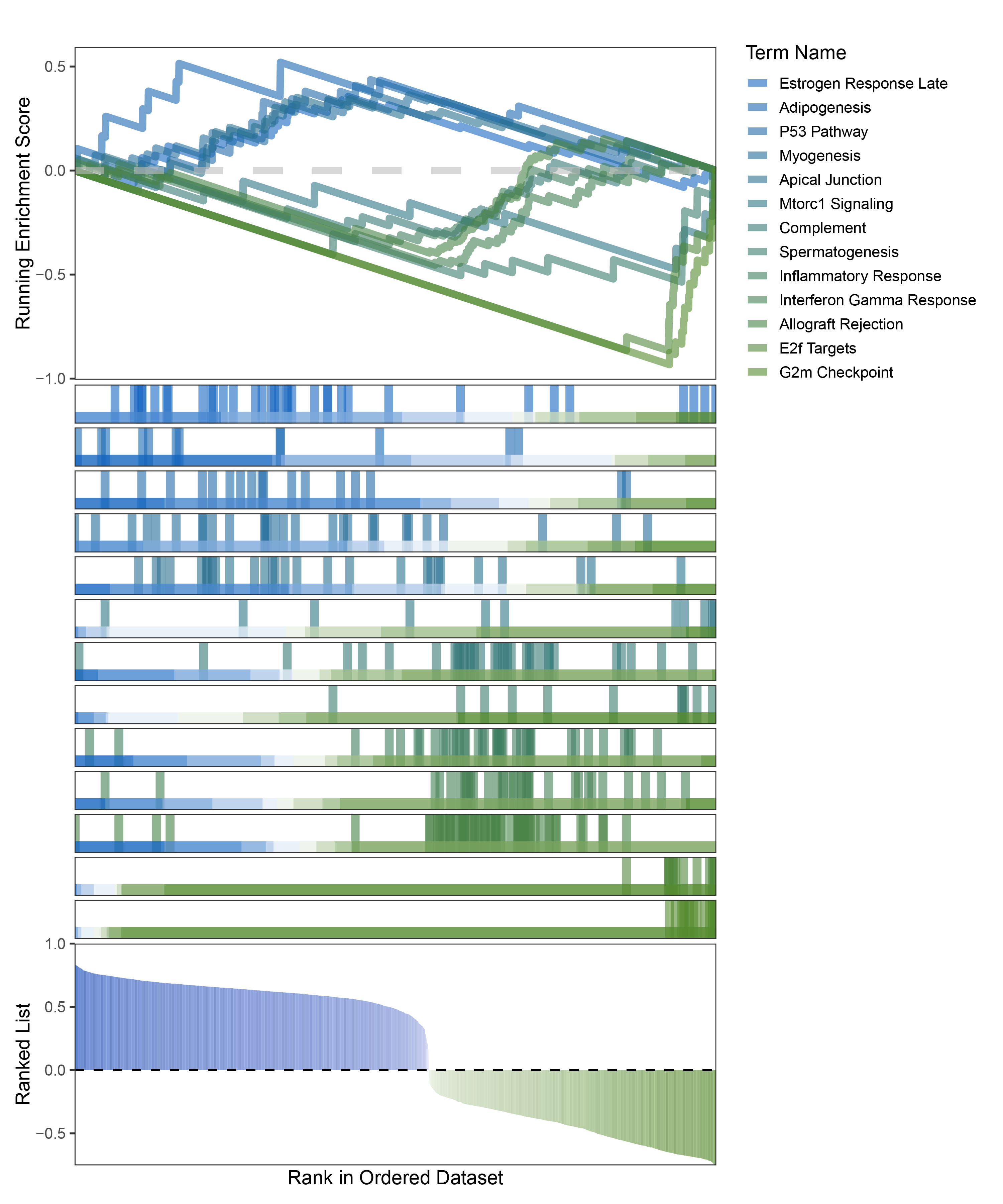
limma_CFD_hallmarks_GSEA_legend

12.1.4.2 KEGG

#kegg
kegg <- read.gmt("c2.cp.kegg.v7.4.symbols.gmt")

limma_CFD_kegg_y <- GSEA(geneList, TERM2GENE = kegg)

# Sort by NES
limmasorted_df <- limma_CFD_kegg_y@result %>% arrange(desc(NES))
# Count the number of core enriched genes per row
limmasorted_df$core_gene_count <- sapply(strsplit(as.character(limmasorted_df$core_enrichment), "/"), length)

# Define a function to process strings (change pathway name prefix and case)
process_string <- function(s) {
  # Remove the first word and underscore at the beginning
  s <- sub("^KEGG_", "", s)
  # Split the string by underscore
  words <- unlist(strsplit(s, "_"))
  # Capitalize the first letter of each word, make other letters lowercase
  words <- tolower(words)
  words <- paste(toupper(substring(words, 1, 1)), substring(words, 2), sep = "")
  # Combine words
  result <- paste(words, collapse = " ")
  return(result)
}

# Apply the function to ID and Description columns
limmasorted_df$ID <- sapply(limmasorted_df$ID, process_string)
limmasorted_df$Description <- sapply(limmasorted_df$Description, process_string)
# Process row names
rownames(limmasorted_df) <- sapply(rownames(limmasorted_df), process_string)
# Display results
print(limmasorted_df)

# Send the processed data back to y@result for easy GSEA pathway diagram
limma_CFD_kegg_y@result <- limmasorted_df

# Process y@geneSets for easy GSEA pathway diagram
# Get the current geneSets names
gene_set_names <- names(limma_CFD_kegg_y@geneSets)
# Apply the process_string function to names
new_gene_set_names <- sapply(gene_set_names, process_string)
# Update the names of geneSets
names(limma_CFD_kegg_y@geneSets) <- new_gene_set_names
# Display the updated geneSets names
print(names(limma_CFD_kegg_y@geneSets))

# Write the result to a CSV file
# write.table(y@result, file="Transpropy_KEGG_GSEA_all.csv", sep=",", row.names=T)

# Display IDs
print(limma_CFD_kegg_y@result$ID)
# Define a color gradient
color = colorRampPalette(c("#1565c0", "#558b2f"))(12)

# Plot all in one image
new_gseaNb(object = limma_CFD_kegg_y,
            geneSetID = c("Arachidonic Acid Metabolism",
                          "Steroid Hormone Biosynthesis",
                          "Metabolism Of Xenobiotics By Cytochrome P450",
                          "Chemokine Signaling Pathway",
                          "Systemic Lupus Erythematosus",
                          "Primary Immunodeficiency",
                          "Leishmania Infection",
                          "Hematopoietic Cell Lineage",
                          "Allograft Rejection",
                          "Graft Versus Host Disease",
                          "Autoimmune Thyroid Disease",
                          "Type I Diabetes Mellitus"), 
            curveCol = color,
            lineSize = 2.5,            # Control the line size of the first plot
            lineAlpha = 0.6,           # Control the transparency of the line in the first plot
            segmentSize = 3,           # Control the size of the vertical lines in the second plot
            segmentAlpha = 0.6,        # Control the transparency of the vertical lines in the second plot
            plotHeightRatio = c(0.3, 0.5, 0.2),  # Control the height ratio of the three plots
            #legend.position = "none",
            htCol = rev(c("#1565c0", "#558b2f")), 
            rankandRev = rev(c("#1565c0", "white", "#558b2f"))
)

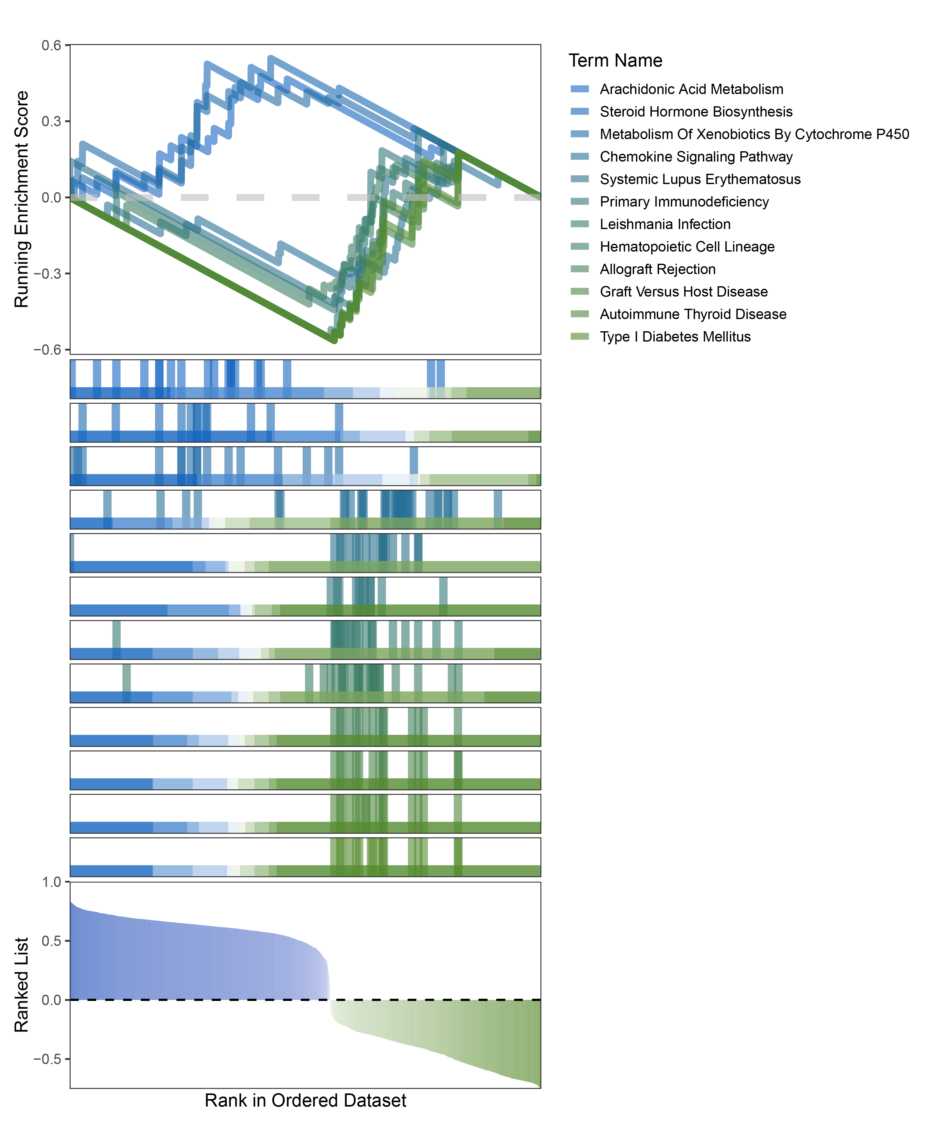
limma_CFD_kegg_GSEA_legend

12.1.5 correlation_outRst_CFD

12.1.5.1 HALLMARKS

geneList <- correlation_outRst_CFD$cor
names(geneList) = correlation_outRst_CFD$gene2
geneList = sort(geneList, decreasing = TRUE)
head(geneList)

#hallmark
hallmarks <- read.gmt("h.all.v7.4.symbols.gmt")
outRst_CFD_hallmarks_y <- GSEA(geneList, TERM2GENE = hallmarks, pvalueCutoff = 0.05)
# Sort by NES
outRstsorted_df <- outRst_CFD_hallmarks_y@result %>% arrange(desc(NES))
# Count the number of core enriched genes per row
outRstsorted_df$core_gene_count <- sapply(strsplit(as.character(outRstsorted_df$core_enrichment), "/"), length)

# Define a function to process strings (change pathway name prefix and case)
process_string <- function(s) {
  # Remove the first word and underscore at the beginning
  s <- sub("^HALLMARK_", "", s)
  # Split the string by underscore
  words <- unlist(strsplit(s, "_"))
  # Capitalize the first letter of each word, make other letters lowercase
  words <- tolower(words)
  words <- paste(toupper(substring(words, 1, 1)), substring(words, 2), sep = "")
  # Combine words
  result <- paste(words, collapse = " ")
  return(result)
}

# Apply the function to ID and Description columns
outRstsorted_df$ID <- sapply(outRstsorted_df$ID, process_string)
outRstsorted_df$Description <- sapply(outRstsorted_df$Description, process_string)
# Process row names
rownames(outRstsorted_df) <- sapply(rownames(outRstsorted_df), process_string)
# Display results
print(outRstsorted_df)

# Send the processed data back to y@result for easy GSEA pathway diagram
outRst_CFD_hallmarks_y@result <- outRstsorted_df

# Process y@geneSets for easy GSEA pathway diagram
# Get the current geneSets names
gene_set_names <- names(outRst_CFD_hallmarks_y@geneSets)
# Apply the process_string function to names
new_gene_set_names <- sapply(gene_set_names, process_string)
# Update the names of geneSets
names(outRgr_CFD_hallmarks_y@geneSets) <- new_gene_set_names
# Display the updated geneSets names
print(names(outRst_CFD_hallmarks_y@geneSets))

# Write the result to a CSV file
# write.table(TransPropysorted_df, file="TransPropy_HALLMARKS_GSEA_all.csv", sep=",", row.names=F)

# Display IDs
print(outRst_CFD_hallmarks_y@result$ID)
# Define a color gradient
color = colorRampPalette(c("#0277bd","#9e9d24"))(8)

# Plot all in one image
new_gseaNb(object = outRst_CFD_hallmarks_y,
            geneSetID = c("Estrogen Response Late",
                          "Il2 Stat5 Signaling",
                          "Inflammatory Response",
                          "Complement",
                          "Interferon Alpha Response",
                          "Il6 Jak Stat3 Signaling",
                          "Interferon Gamma Response",
                          "Allograft Rejection"),
            curveCol = color,
            lineSize = 2.5,            # Control the line size of the first plot
            lineAlpha = 0.7,           # Control the transparency of the line in the first plot
            segmentSize = 3,           # Control the size of the vertical lines in the second plot
            segmentAlpha = 0.7,        # Control the transparency of the vertical lines in the second plot
            plotHeightRatio = c(0.3, 0.5, 0.2),  # Control the height ratio of the three plots
            #legend.position = "none",
            htCol = rev(c("#0277bd","#9e9d24")), 
            rankCol = rev(c("#0277bd","white","#9e9d24"))
)

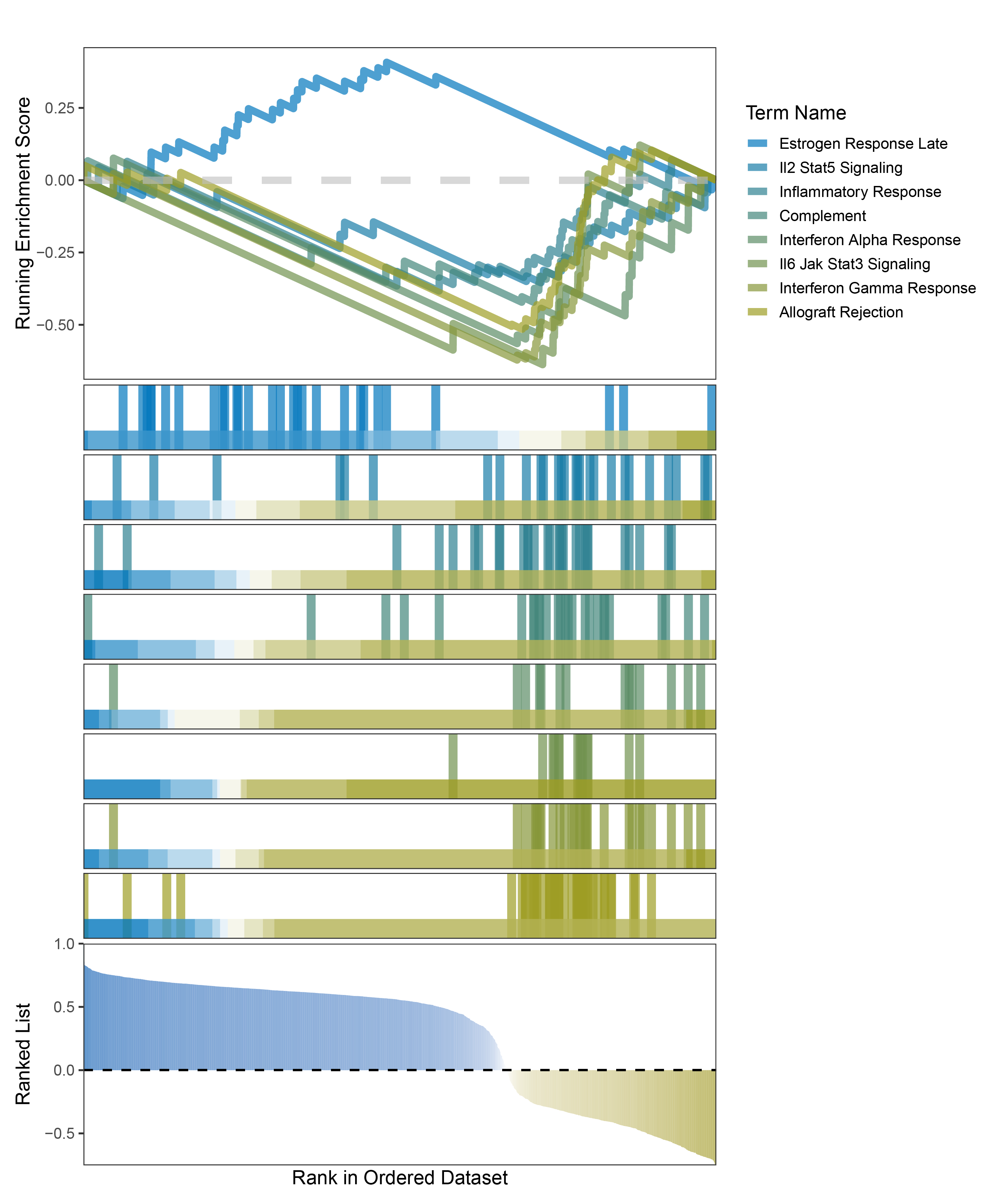
outRst_CFD_hallmarks_GSEA_legend

12.1.5.2 KEGG

#kegg
kegg <- read.gmt("c2.cp.kegg.v7.4.symbols.gmt")

outRst_CFD_kegg_y <- GSEA(geneList, TERM2GENE = kegg)

# Sort by NES
outRstsorted_df <- outRst_CFD_kegg_y@result %>% arrange(desc(NES))
# Count the number of core enriched genes per row
outRstsorted_df$core_gene_count <- sapply(strsplit(as.character(outRstsorted_df$core_enrichment), "/"), length)

# Define a function to process strings (change pathway name prefix and case)
process_string <- function(s) {
  # Remove the first word and underscore at the beginning
  s <- sub("^KEGG_", "", s)
  # Split the string by underscore
  words <- unlist(strsplit(s, "_"))
  # Capitalize the first letter of each word, make other letters lowercase
  words <- tolower(words)
  words <- paste(toupper(substring(words, 1, 1)), substring(words, 2), sep = "")
  # Combine words
  result <- paste(words, collapse = " ")
  return(result)
}

# Apply the function to ID and Description columns
outRstsorted_df$ID <- sapply(outRstsorted_df$ID, process_string)
outRstsorted_df$Description <- sapply(outRstsorted_df$Description, process_string)
# Process row names
rownames(outRstsorted_df) <- sapply(rownames(outRstsorted_df), process_string)
# Display results
print(outRstsorted_df)

# Send the processed data back to y@result for easy GSEA pathway visualization
outRst_CFD_kegg_y@result <- outRstsorted_df

# Process y@geneSets for easy GSEA pathway visualization
# Get the current geneSets names
gene_set_names <- names(outRst_CFD_kegg_y@geneSets)
# Apply the process_string function to names
new_gene_set_names <- sapply(gene_set_names, process_string)
# Update the names of geneSets
names(outRst_CFD_kegg_y@geneSets) <- new_gene_set_names
# Display the updated geneSets names
print(names(outRst_CFD_kegg_y@geneSets))

# Write the result to a CSV file
# write.table(y@result, file="Transpropy_KEGG_GSEA_all.csv", sep=",", row.names=T)

# Display IDs
print(outRst_CFD_kegg_y@result$ID)
# Define a color gradient
color = colorRampPalette(c("#0277bd", "#9e9d24"))(13)

# Plot all in one image
new_gseaNb(object = outRst_CFD_kegg_y,
            geneSetID = c("Steroid Hormone Biosynthesis",
                          "Toll Like Receptor Signaling Pathway",     
                          "Leishmania Infection",
                          "Antigen Processing And Presentation",      
                          "Cell Adhesion Molecules Cams",
                          "Hematopoietic Cell Lineage",               
                          "Natural Killer Cell Mediated Cytotoxicity",
                          "Autoimmune Thyroid Disease",               
                          "Systemic Lupus Erythematosus",
                          "Chemokine Signaling Pathway",              
                          "Allograft Rejection",
                          "Graft Versus Host Disease",                
                          "Type I Diabetes Mellitus"), 
            curveCol = color,
            lineSize = 2.5,            # Control the line size of the first plot
            lineAlpha = 0.7,         # Control the transparency of the first plot's lines
            segmentSize = 3,       # Control the size of the vertical lines in the second plot
            segmentAlpha = 0.7,      # Control the transparency of the vertical lines in the second plot
            plotHeightRatio = c(0.3, 0.5, 0.2),  # Control the height ratio of the three plots
            #legend.position = "none",
            htCol = rev(c("#0277bd", "#9e9d24")), 
            rankCol = rev(c("#0277bd", "white", "#9e9d24"))
)

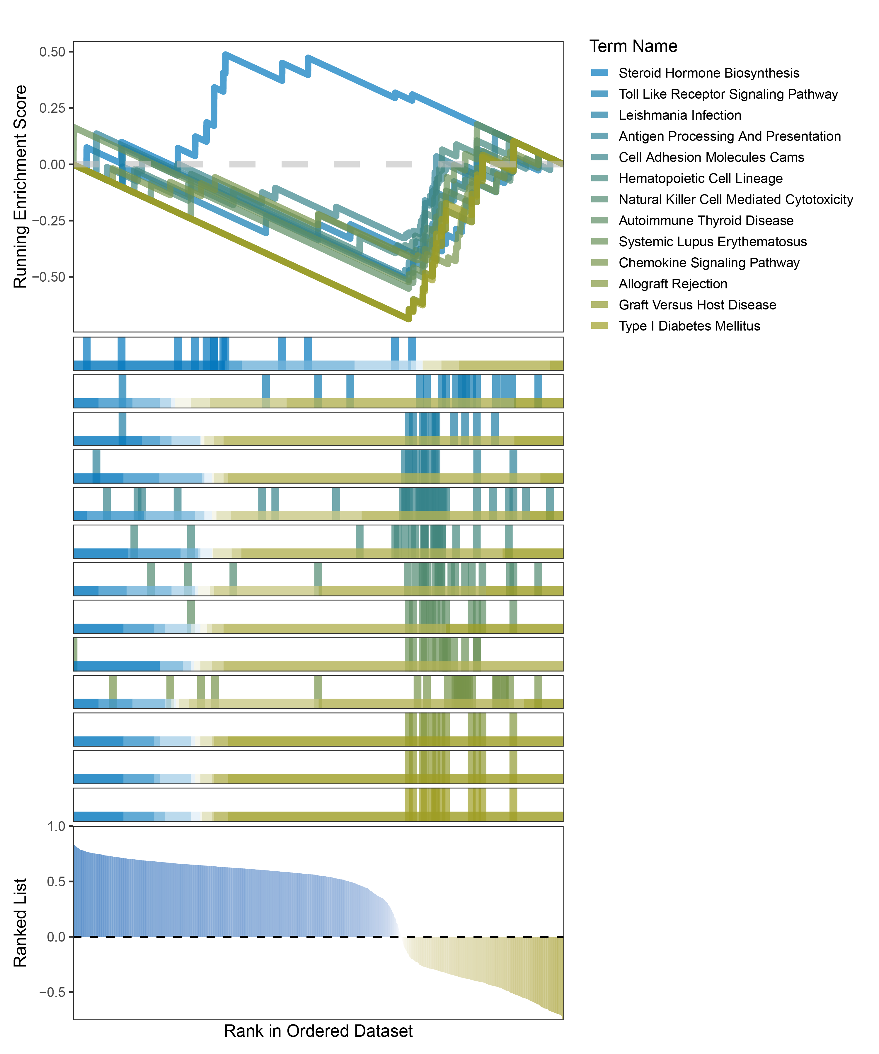
outRst_CFD_kegg_GSEA_legend

12.2 CFD_KEGG_HALLMARKS_ALL

CFD_KEGG_HALLMARKS_ALL

12.3 Discussion

deseq2/edgeR

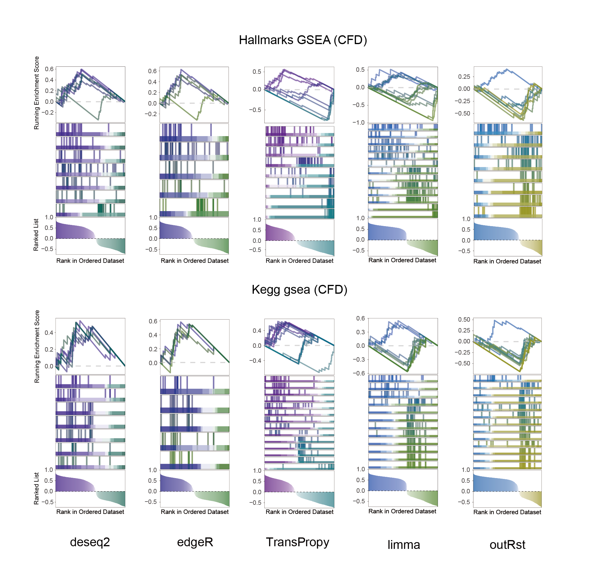
In the Ranked List, the proportion of positively correlated genes is greater than that of negatively correlated ones. Although the proportions of positive and negative values in edgeR are roughly equal, the proportion of genes with absolute correlation values greater than 0.5 remains higher for positive values. GSEA analysis shows a similar trend, with significantly more activated pathways (NES > 0) than inhibited pathways (NES < 0). Pathways enriched for inhibition are very few (or even none), indicating a significant bias in the pathway analysis results.

TransPropy

The proportion of positive and negative genes is balanced, and the proportion of activated and inhibited pathways is also moderate. This avoids the polarization trend seen with other methods. Additionally, the proportions of activated and inhibited pathways are consistent with the trend of positive and negative correlated genes.（Best）

limma/outRst

In the Ranked List, positively correlated genes are more abundant than negatively correlated ones, which is consistent with the results of deseq2 and edgeR. However, GSEA analysis shows the opposite trend, with fewer activated pathways (NES > 0) than inhibited pathways (NES < 0). This phenomenon is particularly pronounced in outRst, where the proportion of negatively correlated genes is smaller, yet the number of enriched inhibited pathways is significantly higher. This imbalance in the proportion of positive and negative pathways is contrary to the trend observed in gene correlation.

Further observation and analysis reveal that the pathways enriched using the limma and RST methods often exhibit very similar rankings and numbers of genes (as indicated by the segment distribution in the middle part of each diagram). This suggests that these pathways are likely the same or highly similar, possibly representing different naming conventions or sub-pathways of a certain type, rather than distinct pathways.Strictly speaking, the primary advantage of the limma and RST methods (which aim to enrich as many pathways as possible, with this advantage originally manifested in the number of inhibited pathways in this study) appears less pronounced.